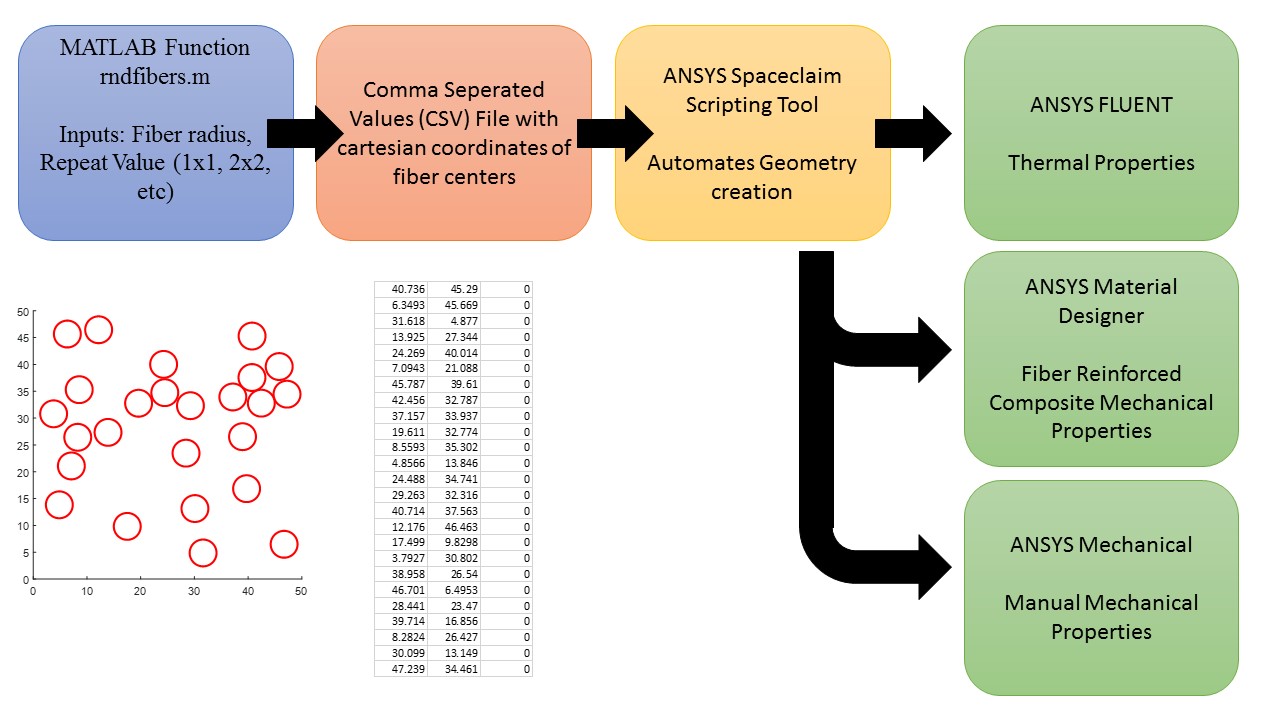
My graduate research focuses on the mechanical and thermal properties of composite materials. The accepted methodology for modeling the behavior of a fiber reinforced composite in an FEM environment usually starts with the development of a representative volume element, or RVE. Drugan and Willis define an RVE as “the smallest material volume element of the composite for which the usual spatially constant ‘overall modulus’ macroscopic constitutive representation is a sufficiently accurate model to represent mean constitutive response.” Development of a RVE allows for accurate models of composite behavior at the laminate and component scales.
To begin studying RVE properties, I first needed to create the geometry of a fiber reinforced composite material in ANSYS. ANSYS has two main geometry programs: Spaceclaim and Design Modeler.
MATLAB Random Fiber Generator
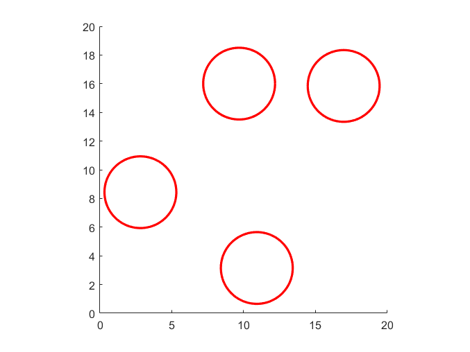
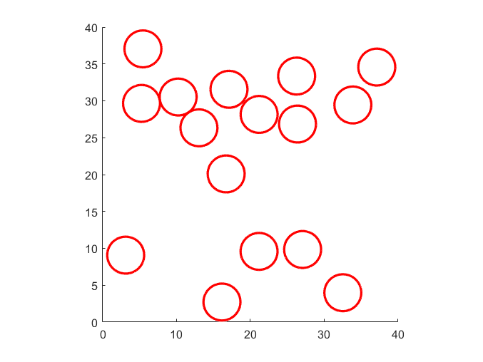
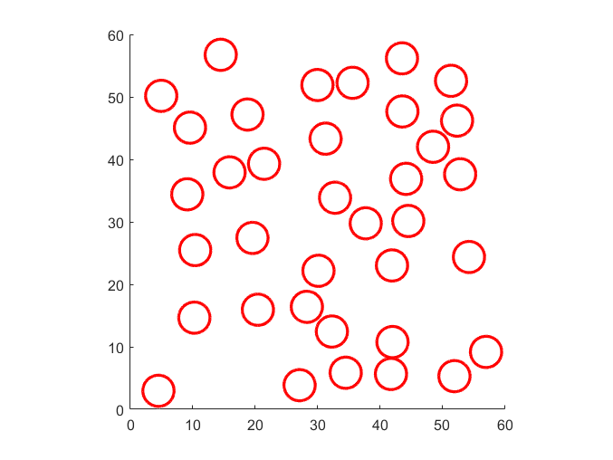
The first step in the fiber modeling is randomly generating a 2D distribution of fibers within a standard geometry. I created the function ‘rndfiber’ in Matlab to achieve this. The ‘rndfiber’ function takes requires two inputs: the radius of the fibers, and the repeat value, which represents the modularity of the RVE. With the base bounding dimension being 10 micrometers (10E-6 m), an inputted repeat value of 5 will output a matrix that is 50 micrometers by 50 micrometers. The number of fibers distributed within the matrix is also determined by the repeat value, and is equal to the repeat value squared. In this example, a repeat value of 5 dictates the creation of 25 individual fibers.
In order to achieve the random distribution of fibers within the specified bounding box, I utilized the ‘rand’ function within Matlab, which returns a uniformly distributed random number in the range [0,1]. Multiplying this by the length and width dimensions scaled the random value to my geometry. However, specific conditions were required to make the geometry easier for analysis. Firstly, fiber center locations were not permitted within half a radius of any of the four edges. This prevented any partial fibers or fibers in contact with the boundaries. Additionally, fiber center locations could not be touching or superimposed on one another. This required calculating the cartesian distance between center points and making sure it was greater than the fiber diameter. All of this was done in a for loop for each required fiber.
After the completion of this loop, all fiber center points are established. For user visualization purposes, the ‘viscircles’ function is used to output an image of the random distribution. Examples can be seen below for different repeat values. Finally, the ‘csvwrite’ function is used to create a comma separated values (CSV) file containing three columns containing the x value, y value, and z value (trivial for now) of each fiber. This CSV file can be opened in Microsoft Excel to verify the success of the file writing.
The Matlab code for the ‘rndfiber’ function is shown below.
function [fiber_x, fiber_y] = rndfiber(r_fiber, repeat)
%Create a random fiber distribution within a matrix and output coordinates

base_dim = 10; %all units assumed to be *10^-6
len = base_dim*repeat;
num_fiber = repeat^2;

fiber_x = [0];
fiber_y = [0];
coordinate_matrix = [0;0];

for i = 1:num_fiber
    x = len*rand(1);
    y = len*rand(1);
    coord = [x;y];

    if i>1
        d_vec = [];
        for j = 1:i-1
            %Calculate the distance between each fiber generated
            d = sqrt((x-coordinate_matrix(1,j))^2 + (y-coordinate_matrix(2,j))^2);
            d_vec = [d_vec d];
        end

        neg_dist = any(d_vec< 2*r_fiber);
        %If any fibers are too close to each other, neg_dist becomes true
    else
        neg_dist = false;

    end

        while neg_dist || x < r_fiber || x > len-r_fiber %wall conditions
            x = len*rand(1);
            d_vec = [];
        for j = 1:i-1
            d = sqrt((x-coordinate_matrix(1,j))^2 + (y-coordinate_matrix(2,j))^2);
            d_vec = [d_vec d];
        end

        neg_dist = any(d_vec< 2*r_fiber);

        end


        while neg_dist || y < r_fiber || y > len-r_fiber
            y = len*rand(1);
%             b = abs(fiber_y-y)-r_fiber;
%             any_ynegatives = any(b<0);
        end


    if i == 1
        coordinate_matrix(1,1) = x;
        coordinate_matrix(2,1) = y;
    else
        coordinate_matrix(1,i) = x;
        coordinate_matrix(2,i) = y;
    end
end


cla
center = [coordinate_matrix(1,:) ; coordinate_matrix(2,:)]';
radii = zeros(1, length(coordinate_matrix));
radii(1:end) = r_fiber;
viscircles(center, radii) %Plot circles
% scatter(fiber_x, fiber_y)
axis square
xlim([0 len])
ylim([0 len])

csv_matrix = [coordinate_matrix(1,:)' coordinate_matrix(2,:)' zeros(1,num_fiber)'];
%output csv file
csvwrite('Fiber_Loc.csv', csv_matrix)
end


ANSYS Spaceclaim
The entire goal of this is to make geometry creation easier for representative volume elements of fiber reinforced composite materials, because I will be modeling them numerous times for research purposes. SpaceClaim is the 3d modeling program packaged within Ansys and what I have used mostly to create geometries. The scripting feature within SpaceClaim is what I leaned on to automate geometry creation. Scripting or macros are a great way to decrease a complicated workflow to a much simpler implementation. Scripting in SpaceClaim uses IronPython, an open source language based on, and extremely similar to Python. It definitely took a week or so to get back up to speed with Python and learn the small distinctions between the two languages. Thankfully, SpaceClaim scripting has a record feature, which when activated turns any actions into code snippets that can replicate exactly what you just did. This recording feature is common in other applications that utilize macros or scripts. I have come across macro recording in both Solidworks and Microsoft Excel. Whatever application you work in, recording is a great way to learn fast as you get direct code representations of the actions you desire to complete.
The ultimate goal of my script is to take in the fiber center points in the CSV file and use them to create a 3d geometry matching the random fiber distribution created in my earlier Matlab function. Without going into excessive detail, my SpaceClaim script starts by creating the 3d bounding box representing the matrix material. After extruding this sketch into a 3d body using the “pull” tool, the code moves into a loop to insert the fibers. The loop utilizes the “combine” tool (misleading, I know) to cut out fibers from the body of the matrix at the coordinate locations inputted in the CSV file. This loop repeats for each fiber until all fibers are represented as bodies in the geometry. Finally, a few more cosmetic changes are done. First, the color of the fiber bodies are changed to more easily visually distinguish them. Lastly, each fiber is lumped into a “named selection” object as “Fiber” and the matrix body is specified as the named selection “Matrix.” While this may seem like a small, pointless action, it is actually one that will save you many headaches further along your modeling journey, as I have learned the hard way. Named Selections get passed into Fleunt, Ansys Mechanical, or whatever other intra-Ansys modeling program utilized. They become important for boundary condition assignments, material assignments, and contour plot visualization to name a few.
