Time Integration Coding Scheme

Problem Statement

A sample material has properties of E=100 GPa, rho=0.3, m(rate sensitivity)= 0.01, and h=1000 MPa. The initial yield stress is 100 MPa. This material undergoes the isochoric deformation process described by

$\LARGE \dot\epsilon_{11}=K, \dot\epsilon_{22}=-K, \dot\epsilon_{33}=\dot\epsilon_{12}=0, \dot\epsilon_{13}=\dot\epsilon_{23}=0.5K \newline$

where

$\newline$ $0 \leq t < 10, \ K = 0.002\ s^{-1} \newline 10 \leq t < 30, \ K = -0.001\ s^{-1} \newline 30 \leq t < 40, \ K = 0.001\ s^{-1}$

Code

This MATLAB Script I developed compares explicit and implicit solution methods. The explicit method solves equations for $\sigma(t)$ and $s(t)$ at each time step in order to update the stress-strain response in the 1-1, 2-2, and 2-3 directions. The implicit method solves the two equations at the current and next time step simultaneously. The implicit method does this by utilizing an initial guess to be updated every iteration, and a multivariate Newton-Raphson method to refine the initial guess based on a given error tolerance. The concern when using either method is getting solutions to converge. The tradeoff between the rigor of each methodology and the size of time step needed to converge becomes quickly apparent.

% ME 6203 Time Integration Scheme
% Pierce Heintzelman
clear
clc
clf
% Start with explicit scheme

% Known Constants
E = 100e9; %Pa
nu = 0.3;

% Shear Modulus
mu=E/2/(1+nu);
k = E/3/(1-2*nu);
lam = k-2/3*mu;

% Tensor - Reduced Form 6x6
C=[[lam+2*mu,lam,lam,0,0,0];[lam,lam+2*mu,lam,0,0,0];...
    [lam,lam,lam+2*mu,0,0,0];[0,0,0,2*mu,0,0];...
    [0,0,0,0,2*mu,0];[0,0,0,0,0,2*mu]];


% plasticity parameters
edot = 0.001;
m = 0.01;
h = 1000e6; %Pa
so = 100e6; %Initial Yield Stress in PA

% Initial strain based on problem statemnt
eo = [.002*ones(1000,1)', -.001*ones(1000,1)', -.001*ones(1000,1)',...
    .001*ones(1000,1)'];

% Initialize stress
sigma0 = [0,0,0,0,0,0]';

ttime = 40;

dtime = ttime/length(eo);
t = dtime:dtime:40;
%Initialize arrays
sig11 = zeros(length(eo),1);
sig22 = zeros(length(eo),1);
sig23 = zeros(length(eo),1);
e11 = zeros(length(eo),1);
e22 = zeros(length(eo),1);
e23 = zeros(length(eo),1);

tic
for i = 1:length(eo)
    if i == 1
        sigma_t = sigma0;
        s_t = so;
    end
    sig11(i) = sigma_t(1);
    sig22(i) = sigma_t(2);
    sig23(i) = sigma_t(6);
    
    
    erate = [eo(i),-1*eo(i), 0, 0, 0.5*eo(i), 0.5*eo(i)]';
    
    % Keeping track of strain
    if i>=2
        e11(i) = e11(i-1) + erate(1)*dtime;
        e22(i) = e22(i-1) + erate(2)*dtime;
        e23(i) = e23(i-1) + erate(6)*dtime;
    end
       
    mises_t = sqrt(0.5*((sigma_t(1)-sigma_t(2))^2 +...
    (sigma_t(2) - sigma_t(3))^2 ...
        + (sigma_t(1) - sigma_t(3))^2+3*(sigma_t(4)^2+sigma_t(5)^2+...
    sigma_t(6)^2)));
    peeqdot = edot * (mises_t/s_t)^(1/m);
    press = (sigma_t(1) + sigma_t(2) + sigma_t(3))/3;
    dev_t = sigma_t - press*[1,1,1,0,0,0]';
    if mises_t==0
        epdot = [0,0,0,0,0,0]';
    else
        epdot = 3/2*peeqdot*dev_t/mises_t;
    end
    % update stress and strength values
    
    sigma_tau = C * (erate-epdot)*dtime + sigma_t;
    sigma_t = sigma_tau;
    s_tau = h*peeqdot*dtime + s_t;
    s_t = s_tau;
     
end
toc
hold on

figure(1)
plot(e11, sig11)

figure(2)
plot(e22, sig22)

figure(3)
plot(e23, sig23)

figure(4)
plot(t, sig11, t, sig22, t, sig23)
xlabel('Time [s]')
ylabel('Stress [Pa]')
legend('11 Direction','22 Direction', '23 Direction', 'Location', 'northwest')
ylim([-1.1e8 1.1e8])

%DT = .001
% Initial strain based on problem statemnt
eo = [.002*ones(10000,1)', -.001*ones(10000,1)', -.001*ones(10000,1)',...
    .001*ones(10000,1)'];

% Initialize stress
sigma0 = [0,0,0,0,0,0]';

ttime = 40;

dtime = ttime/length(eo);
t = dtime:dtime:40;
%Initialize arrays
sig11 = zeros(length(eo),1);
sig22 = zeros(length(eo),1);
sig23 = zeros(length(eo),1);
e11 = zeros(length(eo),1);
e22 = zeros(length(eo),1);
e23 = zeros(length(eo),1);

tic
for i = 1:length(eo)
    if i == 1
        sigma_t = sigma0;
        s_t = so;
    end
    sig11(i) = sigma_t(1);
    sig22(i) = sigma_t(2);
    sig23(i) = sigma_t(6);
    
    
    erate = [eo(i),-1*eo(i), 0, 0, 0.5*eo(i), 0.5*eo(i)]';
    
    % Keeping track of strain
    if i>=2
        e11(i) = e11(i-1) + erate(1)*dtime;
        e22(i) = e22(i-1) + erate(2)*dtime;
        e23(i) = e23(i-1) + erate(6)*dtime;
    end
       
    mises_t = sqrt(0.5*((sigma_t(1)-sigma_t(2))^2 +...
    (sigma_t(2) - sigma_t(3))^2 ...
        + (sigma_t(1) - sigma_t(3))^2+3*(sigma_t(4)^2+...
    sigma_t(5)^2+sigma_t(6)^2)));
    peeqdot = edot * (mises_t/s_t)^(1/m);
    press = (sigma_t(1) + sigma_t(2) + sigma_t(3))/3;
    dev_t = sigma_t - press*[1,1,1,0,0,0]';
    if mises_t==0
        epdot = [0,0,0,0,0,0]';
    else
        epdot = 3/2*peeqdot*dev_t/mises_t;
    end
    % update stress and strength values
    
    sigma_tau = C * (erate-epdot)*dtime + sigma_t;
    sigma_t = sigma_tau;
    s_tau = h*peeqdot*dtime + s_t;
    s_t = s_tau;
     
end
toc 

figure(1)
hold on
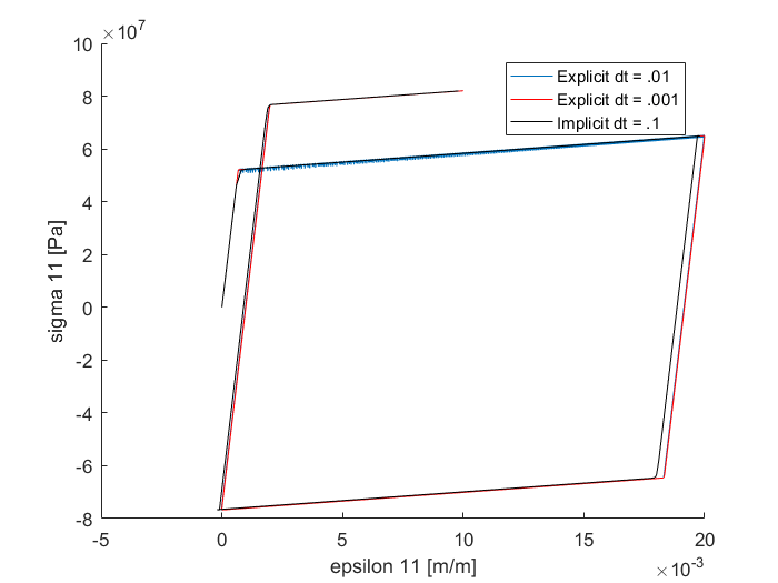
plot(e11, sig11,'r')
xlabel('epsilon 11 [m/m]')
ylabel('sigma 11 [Pa]')
% title('Response in 11 Direction')
legend('Explicit dt = .01','Explicit dt = .001')

figure(2)
hold on
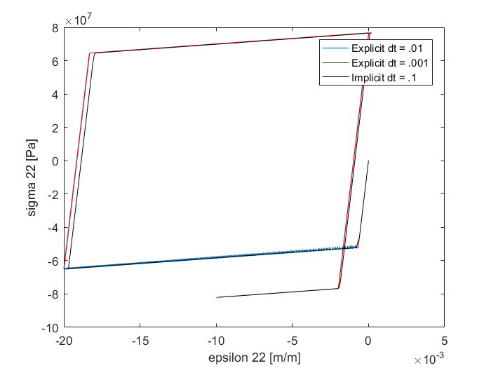
plot(e22, sig22,'r')
xlabel('epsilon 22 [m/m]')
ylabel('sigma 22 [Pa]')
% title('Response in 22 Direction')
legend('Explicit dt = .01','Explicit dt = .001')

figure(3)
hold on
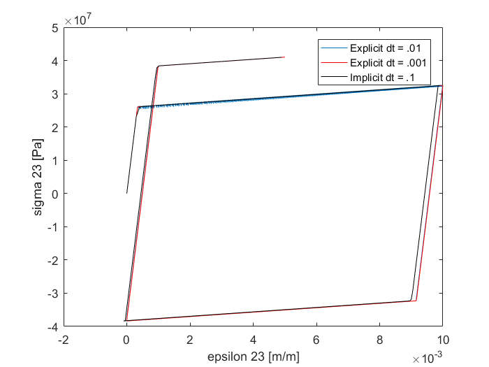
plot(e23, sig23,'r')
xlabel('epsilon 23 [m/m]')
ylabel('sigma 23 [Pa]')
% title('Response in 23 Direction')
legend('Explicit dt = .01','Explicit dt = .001')

figure(5)
plot(t, sig11, t, sig22, t, sig23)
xlabel('Time [s]')
ylabel('Stress [Pa]')
legend('11 Direction','22 Direction', '23 Direction', 'Location', 'northwest')
ylim([-1.1e8 1.1e8])

%Implicit Scheme

%Initialize arrays

eo = [.002*ones(100,1)', -.001*ones(100,1)', -.001*ones(100,1)',...
    .001*ones(100,1)'];

sig11 = zeros(length(eo),1);
sig22 = zeros(length(eo),1);
sig23 = zeros(length(eo),1);
e11 = zeros(length(eo),1);
e22 = zeros(length(eo),1);
e23 = zeros(length(eo),1);


dtime = ttime/length(eo);
t = dtime:dtime:40;

tol = 1e-3; %set tolerance
tic
for i = 1:length(eo)
    if i==1
        sigma_t = sigma0;
        s_t = so;
    end
    sig11(i) = sigma_t(1);
    sig22(i) = sigma_t(2);
    sig23(i) = sigma_t(6);
    
    %strain rate at current time step
    erate = [eo(i),-1*eo(i), 0, 0, 0.5*eo(i), 0.5*eo(i)]';
    
    % strain(tau) = strain(t) + strain_rate*dtime
    if i>=2
        e11(i) = e11(i-1)+erate(1)*dtime;
        e22(i) = e22(i-1)+erate(2)*dtime;
        e23(i) = e23(i-1)+erate(6)*dtime;
    end
    
    %calculate trial stresses - elastic predictor
    sig_tr = C*erate*dtime+sigma_t;
    press = (sig_tr(1) + sig_tr(2) + sig_tr(3))/3;
    dev_tr = sig_tr - press*[1,1,1,0,0,0]';
    
    % Find mises equivalent of t and trial stress
    mises_t = sqrt(0.5*((sigma_t(1)-sigma_t(2))^2 + ...
    (sigma_t(2) - sigma_t(3))^2 ...
        + (sigma_t(1) - sigma_t(3))^2+3*(sigma_t(4)^2+...
    sigma_t(5)^2+sigma_t(6)^2)));
    mises_tr = sqrt(0.5*((sig_tr(1)-sig_tr(2))^2 +...
    (sig_tr(2) - sig_tr(3))^2 ...
        + (sig_tr(1) - sig_tr(3))^2+3*(sig_tr(4)^2+...
    sig_tr(5)^2+sig_tr(6)^2)));
    
   %Newton Raphson iterations
   mises_tau = mises_tr;
   s_tau = s_t;
   for j = 1:500
       peeqdot = edot*(mises_tau/s_tau)^(1/m);
       g1 = mises_tr-mises_tau - 3*mu*peeqdot*dtime;
       g2 = s_tau-s_t-h*peeqdot*dtime;
       g = [g1 g2]';
       y = [mises_tau s_tau]';
       g1m = -1-3*mu*edot*dtime/m*((mises_tau/s_tau)^(1/m-1))/s_tau;
       g1s = 3*mu*dtime/m*peeqdot/s_tau;
       g2m = -1*h*edot*dtime/m*((mises_tau/s_tau)^(1/m-1))/s_tau;
       g2s = 1+h*dtime/m*peeqdot/s_tau;
       J = [[g1m g1s];[g2m g2s]];
       y = y-(inv(J))*g;
       mises_tau = y(1);
       s_tau = y(2);
       if abs(g1)<tol*so && abs(g2) < tol*so
           break           
       end
       if j==50
           disp('Implicit method not converged.')
       end
   end
   corrf = 1+3*mu*edot*dtime*(mises_tau/s_tau)^(1/m-1)/s_tau;
   dev_tau = dev_tr/corrf;
   sigma_tau = dev_tau+press*[1,1,1,0,0,0]';
   
   %stress strength update
   sigma_t = sigma_tau;
   s_t = s_tau; 
      
end
toc

figure(1)
hold on
plot(e11, sig11,'k')
legend('Explicit dt = .01','Explicit dt = .001','Implicit dt = .1')

figure(2)
hold on
plot(e22, sig22,'k')
legend('Explicit dt = .01','Explicit dt = .001','Implicit dt = .1')

figure(3)
hold on
plot(e23, sig23,'k')
legend('Explicit dt = .01','Explicit dt = .001','Implicit dt = .1')

figure(6)
plot(t, sig11, t, sig22, t, sig23)
xlabel('Time [s]')
ylabel('Stress [Pa]')
legend('11 Direction','22 Direction', '23 Direction', 'Location', 'northwest')
ylim([-1.1e8 1.1e8])

Graphical Results

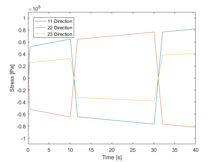
Slide 1: Stress vs Time Implicit Scheme with dt = .1 s

Slide 2: Stress vs Time Explicit Scheme with dt = .01 s

Slide 3: Stress vs Time Explicit Scheme with dt = .001 s

Slide 4: Stress vs Strain in 11 direction

Slide 5: Stress vs Strain in 22 direction

Slide 6: Stress vs Strain in 23 direction

Conclusion

Explicit schemes, while easier to understand conceptually and code, require time steps to converge that are orders of magnitude smaller than those required for implicit schemes. In this problem, a time step 100 times finer was needed for the explicit solution be identical to the implicit solution. Due to these smaller time steps, computation time suffers and therefore implicit schemes should be used in situations where computational efficiency is required. Although implicit schemes are more mathematically rigorous, they are worth the initial effort due to their ease of convergence and decrease in computing time.

Read the full report below

time-integration-coding-scheme-report Download